
Ready to see the future? Let's dive into the art of predicting your sales numbers with a dash of Python wizardry.
In this guide, we'll harness the power of time series forecasting to unveil the secrets of your future sales revenue.
Armed with pandas for data mastery and statsmodels for crafting our crystal ball (aka forecasting model),
we're setting you up to forecast like a pro.
Introduction
Sales forecasting is a crucial part of any business. It helps in making informed decisions about the business for cash flow management, budgeting, and hiring.
At Autohost, we use AWS QuickSight and HubSpot to track our sales revenue. Much of our sales data is stored on S3 and we use AWS Glue to transform and define the schema(s) of the data. This setup allows us to easily experiment with different forecasting models and techniques.
Data Preparation
The first step is to extract the sales data from the database and save it as a CSV file.
We ran the following query on AWS Athena to extract the sales data:
SELECT
    i.user_id AS user_id,
    i.total AS total,
    i.invoice_date AS invoice_date,
    u.integration_source AS integration_name
FROM billing.billing_invoices i
LEFT JOIN autohost.users u
ON u.id = i.user_id
We then saved the result as a CSV file named data.csv.
Data Exploration
We start by creating a new notebook on Google Colab and importing the necessary libraries:
import pandas as pd
import numpy as np
from statsmodels.tsa.statespace.sarimax import SARIMAX
import matplotlib.pyplot as plt
Next, we upload the CSV file to the notebook, load the data into a pandas DataFrame and inspect the first few rows:
# Load your dataset
# Assuming the dataset is stored in a CSV file named 'data.csv'
df = pd.read_csv('data.csv')
df.head()
The output should look something like this:
   user_id  total invoice_date integration_name
0        1  100.0   2023-01-01          Guesty
1        2  200.0   2023-01-01          Cloudbeds
2        3  300.0   2023-01-01          Hostaway
3        4  400.0   2023-01-01          Hospitable
4        5  500.0   2023-01-01          Hostfully
Data Preprocessing
We need to convert the invoice_date column to a datetime object and ensure that the total column is numeric.
# Convert invoice_date to datetime and ensure total is numeric
df['invoice_date'] = pd.to_datetime(df['invoice_date'])
df['total'] = pd.to_numeric(df['total'], errors='coerce')
Next we group the data by date and sum the total sales for each day:
# Aggregate revenue by month (or another period suitable for your analysis)
monthly_revenue = df.groupby(pd.Grouper(key='invoice_date', freq='M')).sum()['total']
Lastly, we fill any missing values with 0:
# Drop any NaN values (if any) to clean up the data
monthly_revenue.fillna(0, inplace=True)
Now, we have a clean dataset with the total sales revenue aggregated by month. Let's visualize the data to make sure it looks as expected.
# Exploratory Data Analysis (optional)
monthly_revenue.plot()
Here's what the plot should look like:
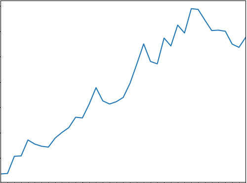
Great! The data looks good and is ready for modeling.
Model Building
We will use the SARIMAX model from the statsmodels library to build our forecasting model.
# Define the model (SARIMAX) - adjust parameters based on your data's seasonality
model = SARIMAX(monthly_revenue, order=(1, 1, 1), seasonal_order=(1, 1, 1, 12))
SARIMAX stands for Seasonal AutoRegressive Integrated Moving Average with eXogenous regressors model. It is a popular and widely used statistical method for time series forecasting.
Next, we fit the model to the data:
# Fit the model
results = model.fit()
Fitting the model means finding the best parameters for the model that minimize the error between the predicted values and the actual values.
Forecasting
Now that we have a fitted model, we can use it to forecast future sales revenue.
# Forecast the next 12 months of revenue
forecast = results.forecast(steps=12)
The forecast variable now contains the predicted sales revenue for the next 12 months.
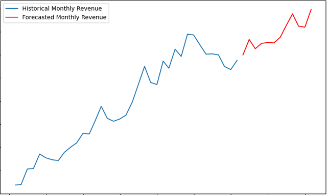
Let's visualize the forecast:
# Plot the historical data and forecast
plt.figure(figsize=(10, 6))
plt.plot(monthly_revenue.index, monthly_revenue, label='Historical Monthly Revenue')
plt.plot(forecast.index, forecast, label='Forecasted Monthly Revenue', color='red')
plt.legend()
plt.show()
The plot should look something like this:
Conclusion
This is an extremely simple example of how to forecast sales revenue using Python. Try creating your own models and experimenting with different parameters to see how the forecasts change. You can also use ChatGPT to help you improve on this example and build more complex models.